42 pivot table excel row labels side by side
How to make row labels on same line in pivot table? - ExtendOffice Make row labels on same line with PivotTable Options, You can also go to the PivotTable Options dialog box to set an option to finish this operation. 1. Click any one cell in the pivot table, and right click to choose PivotTable Options, see screenshot: 2. Excel: How to Sort Pivot Table by Date - Statology Since Excel recognizes the date format, it automatically sorts the pivot table by date from oldest to newest date. However, if we'd like to sort from newest to oldest then we can click on the dropdown arrow next to Row Labels and click Sort Newest to Oldest: The rows in the pivot table will automatically be sorted from newest to oldest: To ...
How to Use Excel Pivot Table Label Filters - Contextures Excel Tips To change the Pivot Table option, and allow multiple filters, follow these steps: Right-click a cell in the pivot table, and click PivotTable Options. In the PivotTable Options dialog box, click the Totals & Filters tab. In the Filters section, add a check mark to 'Allow multiple filters per field.'. Click the OK button, to apply the setting ...

Pivot table excel row labels side by side
How to Customize Your Excel Pivot Chart Data Labels - dummies The Data Labels command on the Design tab's Add Chart Element menu in Excel allows you to label data markers with values from your pivot table. When you click the command button, Excel displays a menu with commands corresponding to locations for the data labels: None, Center, Left, Right, Above, and Below. None signifies that no data labels ... PivotTable Columns Side by Side - Microsoft Community For those who want to know, Just right click each Field in the pivot table and choose Field Settings, go to Layout & Print and select Show item labels in tabular form, Thanx to anyone who is currently composing a response. :0) tod, Report abuse, 6 people found this reply helpful, ·, Was this reply helpful? Yes, No, How to make row labels on same line in pivot table in excel #ExcelMaster, #PivotTable, #ExcelHow to make row labels on same line in pivot table in excelHow to show multiple rows in pivot table in excel
Pivot table excel row labels side by side. Excel Pivot Table with nested rows | Basic Excel Tutorial Steps, 1. Insert your pivot table. Click Insert Menu, under Tables group choose PivotTable. 2. Once you create your pivot table, add all the fields you need to analyze data. How to add the fields, Select the checkbox on each field name you desire in the field section. The selected fields are added to the Row Labels area in the layout section. Multi-row and Multi-column Pivot Table - Excel Start Click OK, Once the pivot table sheet is created, just like in the previous example, drag the Category and the Product to the Rows section and the Sales Value to the Values section to get the same Multi-Row pivot table we did in the previous example. Next we want to add a column. We will add the Date to the Column section by dragging the field. How to Create Excel Pivot Table (Includes practice file) 28.06.2022 · What’s an Excel Pivot Table? You might think of a pivot table as a custom-created summary table of your spreadsheet. It’s a little bit like transpose in Excel, where you can switch your columns and rows.But it also has elements of Excel Tables.And like tables, you can use Excel Slicers to drill down into your data.. You create the pivot table by defining which fields … How to Create a Pivot Table in Excel: A Step-by-Step Tutorial Dec 31, 2021 · After you've completed Step 3, Excel will create a blank pivot table for you. Your next step is to drag and drop a field — labeled according to the names of the columns in your spreadsheet — into the Row Labels area. This will determine what unique identifier — blog post title, product name, and so on — the pivot table will organize ...
Excel Pivot tables 2007 Row labels side by side - MrExcel Message Board Try selecting a cell in the pivot table and then: PivotTable Tools tab, Design tab, Report Layout button in the Layout group, Select "Show in tabular form", J, justjerve, New Member, Joined, Jan 28, 2015, Messages, 1, Jan 28, 2015, #3, Hi Derek Brown and Forrestgump, thank you so much for the question and answer. Pivot table row labels side by side - Excel Tutorials - OfficeTuts Excel You can copy the following table and paste it into your worksheet as Match Destination Formatting. Now, let's create a pivot table ( Insert >> Tables >> Pivot Table) and check all the values in Pivot Table Fields. Fields should look like this. Right-click inside a pivot table and choose PivotTable Options…. Check data as shown on the image below. Pivot table - Wikipedia A pivot table usually consists of row, column and data (or fact) fields.In this case, the column is ship date, the row is region and the data we would like to see is (sum of) units.These fields allow several kinds of aggregations, including: sum, average, standard deviation, count, etc.In this case, the total number of units shipped is displayed here using a sum aggregation. Automate Pivot Table with Python (Create, Filter and Extract) 22.05.2021 · Photo by Jasmine Huang on Unsplash. In Automate Excel with Python, the concepts of the Excel Object Model which contain Objects, Properties, Methods and Events are shared.The tricks to access the Objects, Properties, and Methods in Excel with Python pywin32 library are also explained with examples.. Now, let us leverage the automation of Excel report …
Pivot Table column label from horizontal to vertical Pivot Table column label from horizontal to vertical. After pivot table and with grouping, some column labels have been showed but the caption is on the top. What i want is put the column header at the left of the row as vertical red text show as below. However, i cannot do this, it said "We cant change this part of pivot table". How to add side by side rows in excel pivot table - AnswerTabs To display more pivot table rows side by side, you need to turn on the Classic PivotTable layout and modify Field settings. For example will be used the following table: You have to right-click on pivot table and choose the PivotTable options. Then swich to Display tab and turn on Classic PivotTable layout: 07 Pivot Table side by side row labels - Google Groups - Go to PivotTable Tools, then Options, - in the Active Field, select Field Settings, - In the Field Settings box, select the 2nd tab 'Layout & Print', - Under 'Show item labels in outline form',... Pivot Table Row Labels In the Same Line - Beat Excel! First make a pivot table with required fields. Arrange the fields as shown in left picture. Your initial table will look like right picture. Now click on "Error Code" and access field settings. First check "None" option in "Subtotals & Filters" tab to disable totals after every row.
How To Create A Pivot Table With Multiple Columns And Rows | Awesome Home
How to Format Excel Pivot Table - Contextures Excel Tips Jun 22, 2022 · Video: Change Pivot Table Labels. Watch this short video tutorial to see how to make these changes to the pivot table headings and labels. Get the Sample File. No Macros: To experiment with pivot table styles and formatting, download the sample file. The zipped file is in xlsx format, and and does NOT contain any macros.
Pivot Tables Excel 2007 Row Labels Side By | Brokeasshome.com
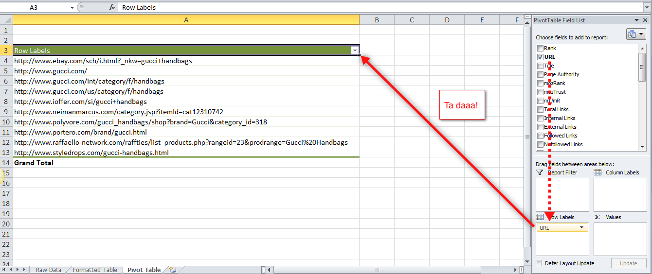
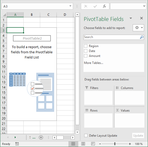
How to Use the Excel Pivot Table Field List - Contextures Excel Tips Apr 19, 2022 · When you create a pivot table, and select a cell in it, by default, a pivot table field list should appear, at the right of the Microsoft Excel window. You can use the field list to select fields for the pivot table layout, and to move pivot table fields to a specific area in the layout.

Excel Pivot Table Report - Sort Data in Row & Column Labels & in Values Area, use Custom Lists
Excel 2007 Pivot Table side by side row labels [SOLVED] Excel 2007 Pivot Table side by side row labels, Hi Masters, In Excel 2003 I could add 2 data elements to the Row label area of the Pivot table. Both items would show up on each row in a different column, this does not happen in 2007 as all items in the row label show up in the same column. How can I revert to the way it was in 2003? Many thanks,
Pivot Table Multiple Row Labels Side By Side | Decorations I Can Make
Pivot Table row labels in separate columns - YouTube 00:00 Pivot table has multiple fields in one column00:15 Change the Pivot Table field to appear in their own columns00:30 Each column is one Pivot Table fiel...

How to Create a Pivot Table in Microsoft Excel | 6 Methods to Try
columns side by side in pivot table - Microsoft Community Replied on July 19, 2017, Drag first name and last name in Rows area and turn off total, if needed, Design tab > Report Layout > Show in Tabular form, Sincerely yours, Vijay A. Verma @ , Report abuse, 16 people found this reply helpful, ·, Was this reply helpful? Yes, No, Question Info,
.jpg)
Excel Pivot Tables Fields in Excel pivot tables Tutorial 02 June 2020 - Learn Excel Pivot Tables ...
Pivot table on excel for macbook air - excelkop The following illustration shows how to move a column field to the row labels area. Right-click a column field, and then click Move to Rows. Right-click a row field, point to Move, and then click Move To Columns. This operation is also called "pivoting" a row or column. When you move a column to a row or a row to a column, you are transposing ...

Repeat all labels in an Excel pivot table | The Right Join
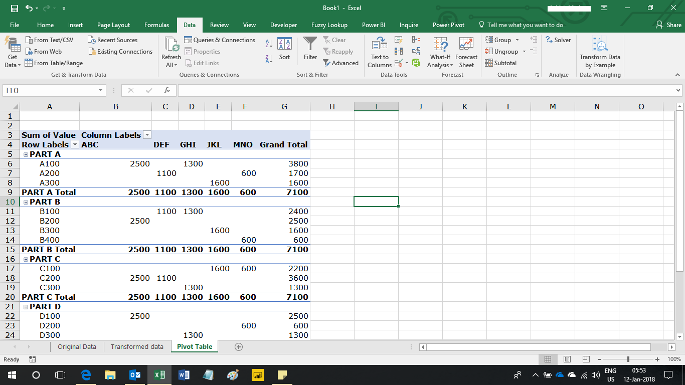
Multi-level Pivot Table in Excel (In Easy Steps) - Excel Easy First, insert a pivot table. Next, drag the following fields to the different areas. 1. Country field to the Rows area. 2. Amount field to the Values area (2x). Note: if you drag the Amount field to the Values area for the second time, Excel also populates the Columns area. Pivot table: 3. Next, click any cell inside the Sum of Amount2 column. 4.
Making Report Layout Changes | Customizing a Pivot Table in Excel 2016 | InformIT
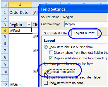
Repeat item labels in a PivotTable - support.microsoft.com Right-click the row or column label you want to repeat, and click Field Settings. Click the Layout & Print tab, and check the Repeat item labels box. Make sure Show item labels in tabular form is selected. Notes: When you edit any of the repeated labels, the changes you make are applied to all other cells with the same label.
multiple fields as row labels on the same level in pivot table Excel - Microsoft Community
How to Add Two-Tier Row Labels to Pivot Tables in Google Sheets Here are the steps to add the second-tier row label as the second column in the Pivot Table: Step 1: Click on any cell in the Pivot Table so that the Pivot table editor sidebar appears on the right side of Google Sheets. Pivot Table, with Pivot table editor sidebar visible. . As you can see, the item column is used as the row labels or ...
Repeat Pivot Table Labels in Excel 2010 - Excel Pivot TablesExcel Pivot Tables
Sort pivot table values with multiple row labels 1. While clicked inside a cell of the pivot table , visit the " Pivot Table Analyze" tab of the ribbon, select the button for "Fields, Items, and Sets," and then click on "Calculated Field.". 2. In the popup, enter the name of the new calculated field (in this case, Jason would name it "profit" or something similar). 3.

How to Sort Pivot Table Row Labels, Column Field Labels and Data Values with Excel VBA Macro ...
Automatic Row And Column Pivot Table Labels - How To Excel At Excel Select the data set you want to use for your table, The first thing to do is put your cursor somewhere in your data list, Select the Insert Tab, Hit Pivot Table icon, Next select Pivot Table option, Select a table or range option, Select to put your Table on a New Worksheet or on the current one, for this tutorial select the first option, Click Ok,
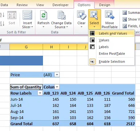
Excel Tip-How To Quickly Select All Or Just Parts Of Your Pivot Table - How To Excel At Excel
The Pivot table tools ribbon in Excel On the right hand side. Choose the fields to start using a pivot table. As you can see when you select any pivot table cell and some tabs glows on the top named Pivot table tools. These two tabs allow you to perform pivot table customization. This is the Pivot table ribbon in Excel. Create pivot table fields , charts and sets.

Excel Pivot Table Tutorial & Sample | Productivity Portfolio
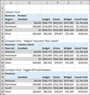
Design the layout and format of a PivotTable To change the format of the PivotTable, you can apply a predefined style, banded rows, and conditional formatting. Windows Web Mac, Changing the layout form of a PivotTable, Change a PivotTable to compact, outline, or tabular form, Change the way item labels are displayed in a layout form, Change the field arrangement in a PivotTable,

Excel Pivot Table Tutorial & Sample | Productivity Portfolio
101 Advanced Pivot Table Tips And Tricks You Need To Know 25.04.2022 · When creating a pivot table it’s usually a good idea to turn your data into an Excel Table. When adding new rows or columns to your source data, you won’t need to update the range reference in your pivot tables if your data is in a Table. Without a table your range reference will look something like above. In this example, if we were to add data past Row 51 …
Discover Pivot Tables – Excel’s most powerful feature and also least known
Pivot table row labels in separate columns • AuditExcel.co.za Our preference is rather that the pivot tables are shown in tabular form (all columns separated and next to each other). You can do this by changing the report format. So when you click in the Pivot Table and click on the DESIGN tab one of the options is the Report Layout. Click on this and change it to Tabular form.

Analyzing Data in Excel
How to Add Rows to a Pivot Table: 9 Steps (with Pictures) - wikiHow 2. Click anywhere in your pivot table. This opens the pivot table editor on the right side of Google Sheets. 3. Click Add under "Rows." It's in the left side of the pivot table editor. A list of fields will expand on the menu. 4. Click the name of the field you want to add as a row.

Excel Pivot Tables: A Comprehensive Guide - HowToAnalyst
How To Compare Multiple Lists of Names with a Pivot Table 08.07.2014 · When we add the Name field to the Rows area of the pivot table (step 2 above), Excel automatically consolidates the list for us and creates a row for each unique name from the combined list. This means that names that appear in multiple years will only be listed once. For example, the name Asher Mays appears three times in the combined list (source data of the …
Post a Comment for "42 pivot table excel row labels side by side"