41 how to add percentage and category name data labels in excel

Custom Chart Data Labels In Excel With Formulas Select the chart label you want to change. In the formula-bar hit = (equals), select the cell reference containing your chart label's data. In this case, the first label is in cell E2. Finally, repeat for all your chart laebls. If you are looking for a way to add custom data labels on your Excel chart, then this blog post is perfect for you. Excel charts: add title, customize chart axis, legend and data labels Click the data series you want to label. To add a label to one data point, click that data point after selecting the series. Click the Chart Elements button, and select the Data Labels option. For example, this is how we can add labels to one of the data series in our Excel chart:

Add a DATA LABEL to ONE POINT on a chart in Excel All the data points will be highlighted. Click again on the single point that you want to add a data label to. Right-click and select ' Add data label '. This is the key step! Right-click again on the data point itself (not the label) and select ' Format data label '. You can now configure the label as required — select the content of ...

How to add percentage and category name data labels in excel

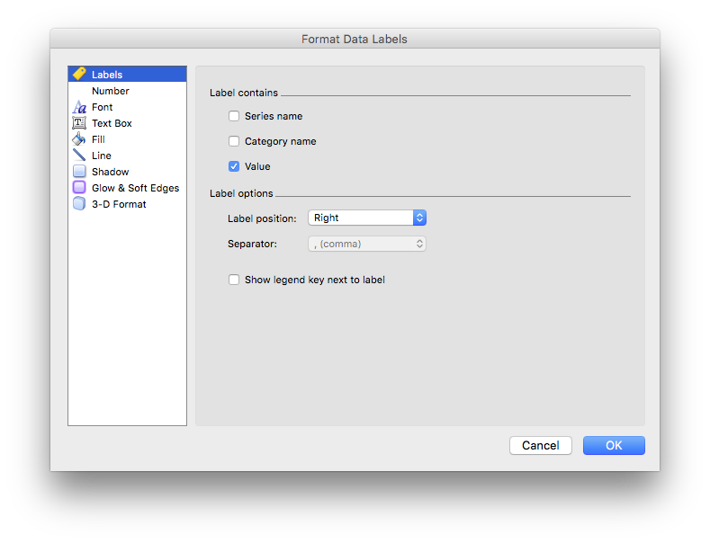
How to show values in data labels of Excel ... - MrExcel Message Board I've made the chart using the first worksheet column for category labels, the second for the bars (percentages), and the third for the line cumulative percentages). I added data labels to the bars, using Excel 2013's option to use label text from cells, referencing the text in the fourth worksheet column. Add or remove data labels in a chart - support.microsoft.com Right-click the data series or data label to display more data for, and then click Format Data Labels. Click Label Options and under Label Contains, pick the options you want. Use cell values as data labels You can use cell values as data labels for your chart. How To Add and Remove Legends In Excel Chart? - EDUCBA If we want to add the legend in the excel chart, it is a quite similar way how we remove the legend in the same way. Select the chart and click on the “+” symbol at the top right corner. From the pop-up menu, give a tick mark to the Legend.

How to add percentage and category name data labels in excel. How to Change Excel Chart Data Labels to Custom Values? First add data labels to the chart (Layout Ribbon > Data Labels) Define the new data label values in a bunch of cells, like this: Now, click on any data label. This will select "all" data labels. Now click once again. At this point excel will select only one data label. How to Add Data Bars in Excel? - EDUCBA We will add excel Data bars for this data which shows the bars inside the cell along with the numbers. Follow the below steps to add data bars in Excel. Step 3: Select the number range from B2 to B11. Step 4: Go to the HOME tab. Select Conditional Formatting and then select Data Bars. Here we have two different categories to highlight; select the first one. Format Number Options for Chart Data Labels in Excel 2011 ... - Indezine Figure 1: Chart with Data Values added as Data Labels. Follow these steps to learn how to format the values used in Data Labels within Excel 2011: Select the chart -- then select the Charts tab which appears on the Ribbon, as shown highlighted in red within Figure 2. Within the Charts tab, click the Edit button (highlighted in blue within ... Excel for Commerce | Analyze large data sets in Excel May 07, 2015 · (In Excel 2013, click on the Add Chart Element button at the left; the procedure is slightly different for other version of Excel). Name the x-axis Years and the y-axis Names per birth and, while you’re at it, change the chart title to Diversity.Ignore the first half of the graph for now: let’s look at 1960 to present.

Excel.ChartDataLabels class - Office Add-ins | Microsoft Docs The request context associated with the object. This connects the add-in's process to the Office host application's process. Specifies the format of chart data labels, which includes fill and font formatting. Specifies the horizontal alignment for chart data label. See Excel.ChartTextHorizontalAlignment for details. How to create a chart with both percentage and value in Excel? 1. Click Kutools > Charts > Category Comparison > Stacked Chart with Percentage, see screenshot: 2. In the Stacked column chart with percentage dialog box, specify the data range, axis labels and legend series from the original data range separately, see screenshot: 3. Add data labels and callouts to charts in Excel 365 - EasyTweaks.com Step #1: After generating the chart in Excel, right-click anywhere within the chart and select Add labels. Note that you can also select the very handy option of Adding data Callouts. Note that you can also select the very handy option of Adding data Callouts. Multiple data labels (in separate locations on chart) Running Excel 2010 2D pie chart I currently have a pie chart that has one data label already set. The Pie chart has the name of the category and value as data labels on the outside of the graph. I now need to add the percentage of the section on the INSIDE of the graph, centered within the pie section. I'm aware that I could type in the percentages as text boxes, but I want this graph to ...

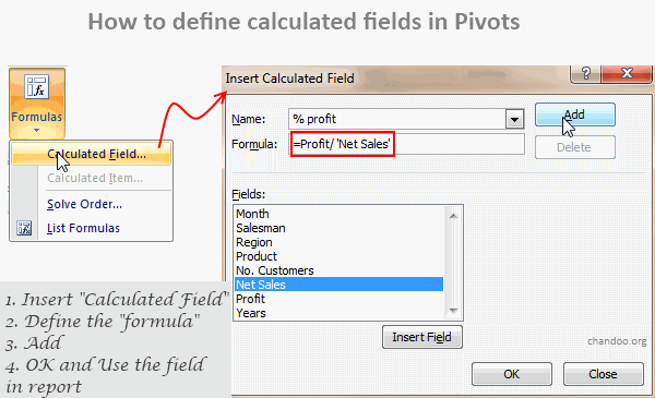
Change the format of data labels in a chart You can add a built-in chart field, such as the series or category name, to the data label. But much more powerful is adding a cell reference with explanatory text or a calculated value. Click the data label, right click it, and then click Insert Data Label Field. If you have selected the entire data series, you won't see this command. How to use Excel Data Model & Relationships - Chandoo.org Jul 01, 2013 · Handling large volumes of data in Excel—Since Excel 2013, the “Data Model” feature in Excel has provided support for larger volumes of data than the 1M row limit per worksheet. Data Model also embraces the Tables, Columns, Relationships representation as first-class objects, as well as delivering pre-built commonly used business scenarios ... Free Budget vs. Actual chart Excel Template - Download May 16, 2018 · Create Budget vs Actual chart with smart labels in Excel – Tutorial. If you are in a hurry to make such a chart, download the template, plug in your values and you are good to go. For instructions on how to create them in Excel, read along. Step 1: Getting the data. Set up your data. Solve Equation in Excel | How to Solve Equation with Solver ... Goal Seek: It is an inbuilt function in excel under What-If Analysis, which helps us solve equations to source cell values until the desired output is achieved. Recommended Articles. This is a guide to Solve Equation in Excel. Here we discuss how to add the Solver Add-in Tool and how to Solve equations with Solver Add-in Tool in excel.

How to Create a Pie Chart in Excel | Smartsheet

excel - How can I add chart data labels with percentage? - Stack Overflow 2. I want to add chart data labels with percentage by default with Excel VBA. Here is my code for creating the chart: Private Sub CommandButton2_Click () ActiveSheet.Shapes.AddChart.Select ActiveChart.SetSourceData Source:=Range ("'Sheet1'!$A$6:$D$6") ActiveChart.ChartType = xlDoughnut End Sub. It only creates Doughnut chart with no information labels.

Excel & Google Sheets Chart Resources That Will Make Your Life Easier | PPC Hero

How to Customize Your Excel Pivot Chart Data Labels - dummies The Data Labels command on the Design tab's Add Chart Element menu in Excel allows you to label data markers with values from your pivot table. When you click the command button, Excel displays a menu with commands corresponding to locations for the data labels: None, Center, Left, Right, Above, and Below. None signifies that no data labels ...

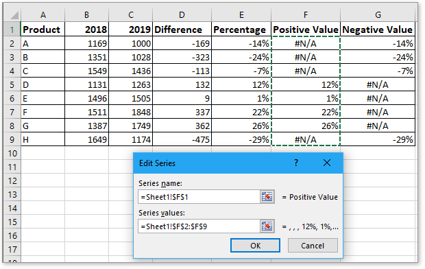
Quickly create a positive negative bar chart in Excel

How to show data label in "percentage" instead of - Microsoft Community Select Format Data Labels. Select Number in the left column. Select Percentage in the popup options. In the Format code field set the number of decimal places required and click Add. (Or if the table data in in percentage format then you can select Link to source.) Click OK

Business Diary: October 2011

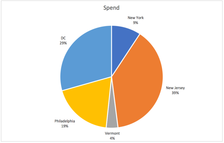
Video: Customize a pie chart - support.microsoft.com In the labels, the dollar amounts are replaced with percentages. I’d also like to show the Salesperson’s name. So, in the pane, I’ll check Category Name. A name and percentage now show in the data label. I’ll click X to close the pane. I like the labels, though the ones at the top are crowded under the title. To fix that, I can rotate ...

Pie Charts bring in Best Presentation for Growth

Excel tutorial: How to use data labels When first enabled, data labels will show only values, but the Label Options area in the format task pane offers many other settings. You can set data labels to show the category name, the series name, and even values from cells. In this case for example, I can display comments from column E using the "value from cells" option. Leader lines simply connect a data label back to a chart element when it's moved. You can turn them off if you want. You can also combine values in data labels and ...

Excel VBA: Pivot Table Tricks to Make You a Star

Adding data labels to a pie chart - Excel General - OzGrid Re: Adding data labels to a pie chart. Thanks again, norie. Really appreciate the help. I tried recording a macro while doing it manually (before my first post). But it didn't record anything about labels, much less making them bold.

Learn SEO The Ultimate Guide For SEO Beginners 2020 - Your Optimized Solutions

How to set and format data labels for Excel charts in C# In label options, we could set whether label contains series name, category name, value, percentages (pie chart) and legend key. This article is going to introduce the method to set and format data labels for Excel charts in C# using Spire.XLS. Note: before start, please download the latest version of Spire.XLS and add the .dll in the bin folder as the reference of Visual Studio. Step 1: Create an Excel document and add sample data.

Working with Charts — XlsxWriter Documentation

Count and Percentage in a Column Chart - ListenData Download the workbook. Steps to show Values and Percentage. 1. Select values placed in range B3:C6 and Insert a 2D Clustered Column Chart (Go to Insert Tab >> Column >> 2D Clustered Column Chart). See the image below. Insert 2D Clustered Column Chart. 2. In cell E3, type =C3*1.15 and paste the formula down till E6.

Share :