45 excel data labels from third column
How to add data labels from different column in an Excel chart? This method will guide you to manually add a data label from a cell of different column at a time in an Excel chart. 1. Right click the data series in the chart, and select Add Data Labels > Add Data Labels from the context menu to add data labels. 2. How to compare two columns and return values from the third column in ... The entire Column C items in Sheet 2 to be compared with first row item in Column A and if any corresponding values/data are there in Column A, then Column B to be populated with data corresponding to the row item in Column D. Column C will have a single word. Column D may or may not have data in it. Column A will have more text.
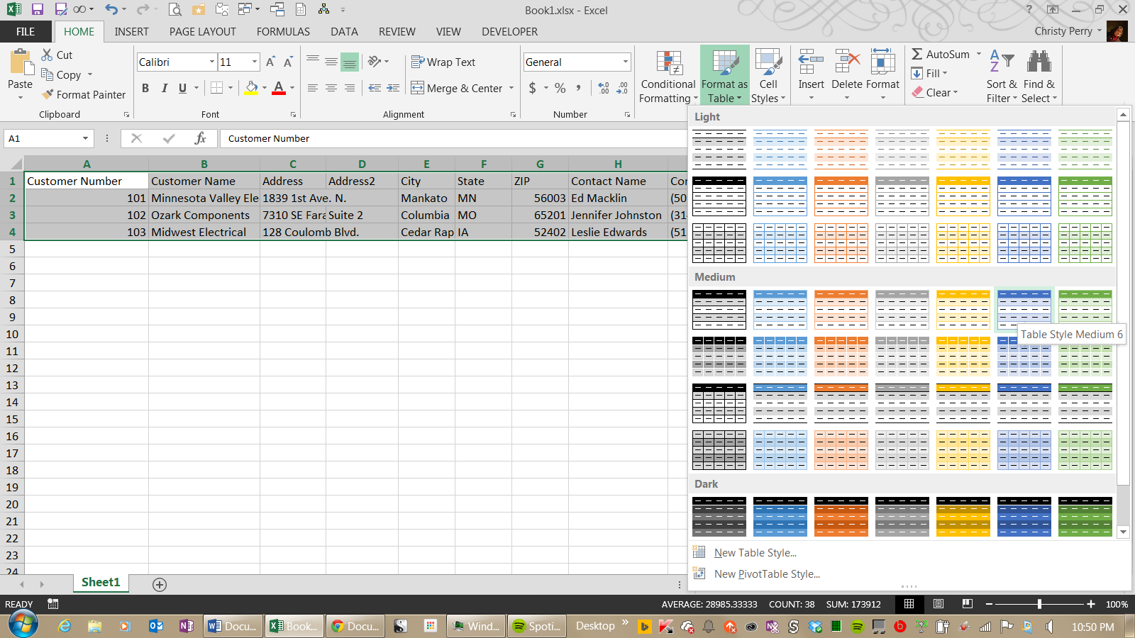
How to Use Cell Values for Excel Chart Labels Select the chart, choose the "Chart Elements" option, click the "Data Labels" arrow, and then "More Options." Uncheck the "Value" box and check the "Value From Cells" box. Select cells C2:C6 to use for the data label range and then click the "OK" button. The values from these cells are now used for the chart data labels.

Excel data labels from third column
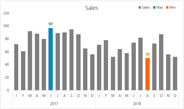
Excel, giving data labels to only the top/bottom X% values 1) Create a data set next to your original series column with only the values you want labels for (again, this can be formula driven to only select the top / bottom n values). See column D below. 2) Add this data series to the chart and show the data labels. 3) Set the line color to No Line, so that it does not appear! 4) Volia! See Below! Share Change the format of data labels in a chart To get there, after adding your data labels, select the data label to format, and then click Chart Elements > Data Labels > More Options. To go to the appropriate area, click one of the four icons ( Fill & Line, Effects, Size & Properties ( Layout & Properties in Outlook or Word), or Label Options) shown here. How to Change Excel Chart Data Labels to Custom Values? You can change data labels and point them to different cells using this little trick. First add data labels to the chart (Layout Ribbon > Data Labels) Define the new data label values in a bunch of cells, like this: Now, click on any data label. This will select "all" data labels. Now click once again.
Excel data labels from third column. 2 data labels per bar? - Microsoft Community Tushar Mehta Replied on January 25, 2011 Use a formula to aggregate the information in a worksheet cell and then link the data label to the worksheet cell. See Data Labels Tushar Mehta (Technology and Operations Consulting) (Excel and PowerPoint add-ins and tutorials) Add or remove data labels in a chart - support.microsoft.com Right-click the data series or data label to display more data for, and then click Format Data Labels. Click Label Options and under Label Contains, select the Values From Cells checkbox. When the Data Label Range dialog box appears, go back to the spreadsheet and select the range for which you want the cell values to display as data labels. How to Create Labels in Word from an Excel Spreadsheet Select Browse in the pane on the right. Choose a folder to save your spreadsheet in, enter a name for your spreadsheet in the File name field, and select Save at the bottom of the window. Close the Excel window. Your Excel spreadsheet is now ready. 2. Configure Labels in Word. How to categorize data based on values in Excel? - ExtendOffice Categorize data based on values with If function. To apply the following formula to categorize the data by value as you need, please do as this: Enter this formula: =IF (A2>90,"High",IF (A2>60,"Medium","Low")) into a blank cell where you want to output the result, and then drag the fill handle down to the cells to fill the formula, and the data ...
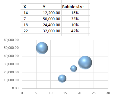
VLOOKUP Hack #4: Column Labels - Excel University The 3rd argument of the VLOOKUP function is officially known as col_index_num. This represents the position of the value you want returned. For example, if you want to return the amount from the 2nd position, or column, within the lookup range, you would enter 2 for the argument. Consider the screenshot below. Add Custom Labels to x-y Scatter plot in Excel Step 1: Select the Data, INSERT -> Recommended Charts -> Scatter chart (3 rd chart will be scatter chart) Let the plotted scatter chart be. Step 2: Click the + symbol and add data labels by clicking it as shown below. Step 3: Now we need to add the flavor names to the label. Now right click on the label and click format data labels. How to Print Labels From Excel - EDUCBA Navigate towards the folder where the excel file is stored in the Select Data Source pop-up window. Select the file in which the labels are stored and click Open. A new pop up box named Confirm Data Source will appear. Click on OK to let the system know that you want to use the data source. Again a pop-up window named Select Table will appear. Apply Custom Data Labels to Charted Points - Peltier Tech Click once on a label to select the series of labels. Click again on a label to select just that specific label. Double click on the label to highlight the text of the label, or just click once to insert the cursor into the existing text. Type the text you want to display in the label, and press the Enter key.
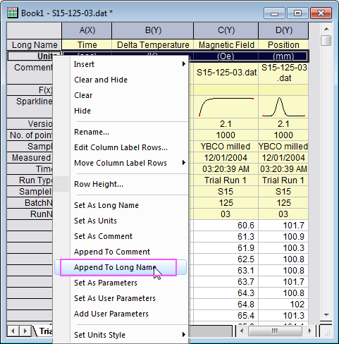
Using a cell contents of a third column of data as data label for each ... Column 1 is a numeric value for an ion and is on the X-axis, column 2 is a numerical value for intensity at the value of column 1. Column 3 is a text descriptor of what type of ion gives that column 1 reading value and its column 2 intensity value. I would like to use the column 3 data to label each column on the chart above the column. How to Add Labels to Scatterplot Points in Excel - Statology Next, click anywhere on the chart until a green plus (+) sign appears in the top right corner. Then click Data Labels, then click More Options… In the Format Data Labels window that appears on the right of the screen, uncheck the box next to Y Value and check the box next to Value From Cells. How do you label data points in Excel? - profitclaims.com Batch add all data labels from different column in an Excel chart. This method will introduce a solution to add all data labels from a different column in an Excel chart at the same time. Please do as follows: 1. Right click the data series in the chart, and select Add Data Labels > Add Data Labels from the context menu to add data labels. 2. Using Data Labels from a Third Data Column in an Chart Excel 2013, allows you to select Data Labels locations from a Dialog box Prior to that it had to be done either manually or via a Macro To do it manually Select a Series Add a Data Label Select the Data Labels Then select an Individual Data Label In the formula bar =$D$2 (Cell reference to your new labels) Repeat for all Labels G guna_sekar87
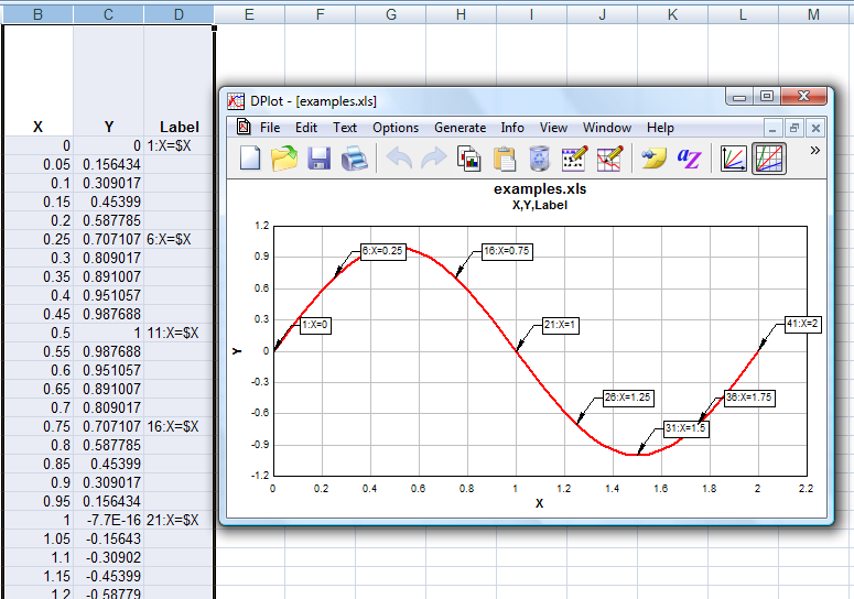
DPlot Windows software for Excel users to create presentation quality graphs
How to Customize Your Excel Pivot Chart Data Labels - dummies To remove the labels, select the None command. If you want to specify what Excel should use for the data label, choose the More Data Labels Options command from the Data Labels menu. Excel displays the Format Data Labels pane. Check the box that corresponds to the bit of pivot table or Excel table information that you want to use as the label.
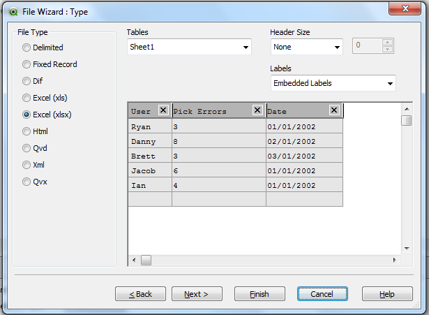
Solved: How to Display Excel sheet Column name - Qlik Community - 769330
How to create Custom Data Labels in Excel Charts To customize it, click on the arrow next to Data Labels and choose More Options … Unselect the Value option and select the Value from Cells option. Choose the third column (without the heading) as the range. Now we have exactly what we want. Some labels may overlap the chart elements and they have a transparent background by default.
How to add data labels from different column in an Excel chart?
Adding rich data labels to charts in Excel 2013 - Microsoft 365 Blog Putting a data label into a shape can add another type of visual emphasis. To add a data label in a shape, select the data point of interest, then right-click it to pull up the context menu. Click Add Data Label, then click Add Data Callout . The result is that your data label will appear in a graphical callout.
Label Columns In Excel - Ythoreccio
Custom Excel Chart Label Positions - My Online Training Hub Custom Excel Chart Label Positions - Setup. The source data table has an extra column for the 'Label' which calculates the maximum of the Actual and Target: The formatting of the Label series is set to 'No fill' and 'No line' making it invisible in the chart, hence the name 'ghost series': The Label Series uses the 'Value ...

Enable or Disable Excel Data Labels at the click of a button - How To - PakAccountants.com
Can you label grouped columns in excel? To do this, select a Row Labels cell or the Column Labels cell that you want to group, right-click your selection, and choose Group from the shortcut menu. Next, right-click the new group and choose Collapse from the shortcut menu. ... How do I consolidate Data in Excel? Click Data>Consolidate (in the Data Tools group). In the Function box ...
Ease the Pain of Data Entry with an Excel Forms Template | Pryor Learning Solutions
Mac Excel 2008 - How to add Data Labels for Scatter Plot coming from ... In Excel 2008, to select X axis for the labels: go to 'Formatting palette' navigate to 'Chart Option' Under 'Other options' select "category name' in Labels. A AsherS New Member Joined Feb 9, 2012 Messages 9 Jul 30, 2014 #3 Cyrilbrd, this does not add a label from another column. This only displays the X-value and does not solve the issue. cyrilbrd

How to Create Multi-Category Chart in Excel - Excel Board
How can I add data labels from a third column to a scatterplot? Do you want to add data labels to the 3rd column values in the chart? Highlight the 3rd column range in the chart. Click the chart, and then click the Chart Layout tab. Under Labels, click Data Labels, and then in the upper part of the list, click the data label type that you want.

How to edit the label of a chart in Excel? - Stack Overflow
Custom Data Labels with Colors and Symbols in Excel Charts - [How To] The way I know is to simply click the data label once and clicking it again will select the particular data label which you can then format with desired color. And of course you will have to do it for each data label separately. Tiring right? And above that it is "hard" coloring the labels.
31 How To Label Excel Columns - Labels Database 2020
How to add data labels to a Column (Vertical Bar) Graph in ... - YouTube Get to know about easy steps to add data labels to a Column (Vertical Bar) Graph in Microsoft® Excel 2010 by watching this video.Content in this video is pro...

How to Create Multi-Category Chart in Excel - Excel Board
Create a multi-level category chart in Excel - ExtendOffice 1.3) In the third column, type in each data for the subcategories. 2. Select the data range, click Insert > Insert Column or Bar Chart > Clustered Bar. 3. Drag the chart border to enlarge the chart area. See the below demo. 4. Right click the bar and select Format Data Series from the right-clicking menu to open the Format Data Series pane.

How to Sort data in Microsoft Excel
How to Change Excel Chart Data Labels to Custom Values? You can change data labels and point them to different cells using this little trick. First add data labels to the chart (Layout Ribbon > Data Labels) Define the new data label values in a bunch of cells, like this: Now, click on any data label. This will select "all" data labels. Now click once again.

Merging 2 spreadsheets on Excel 2010 - Super User
Change the format of data labels in a chart To get there, after adding your data labels, select the data label to format, and then click Chart Elements > Data Labels > More Options. To go to the appropriate area, click one of the four icons ( Fill & Line, Effects, Size & Properties ( Layout & Properties in Outlook or Word), or Label Options) shown here.
:max_bytes(150000):strip_icc()/Capture-f3f27cf55e1d449abb93f0179ef41c3b.JPG)
Change Column Colors / Show Percent Labels in Excel Column Chart
Excel, giving data labels to only the top/bottom X% values 1) Create a data set next to your original series column with only the values you want labels for (again, this can be formula driven to only select the top / bottom n values). See column D below. 2) Add this data series to the chart and show the data labels. 3) Set the line color to No Line, so that it does not appear! 4) Volia! See Below! Share
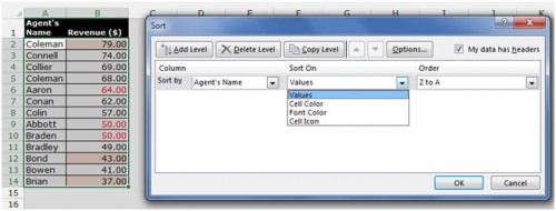
How to Sort data in Microsoft Excel

Business Diary: October 2011
Select data for a chart - Excel

stepping forward to learn excel daily..: Sub - Divided or Component Bar Diagram
Post a Comment for "45 excel data labels from third column"