43 how to change excel chart data labels to custom values

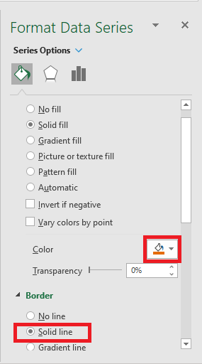
Change the format of data labels in a chart To format data labels, select your chart, and then in the Chart Design tab, click Add Chart Element > Data Labels > More Data Label Options. Click Label Options and under Label Contains, pick the options you want. To make data labels easier to read, you can move them inside the data points or even outside of the chart. How to add data labels from different column in an Excel ... This method will guide you to manually add a data label from a cell of different column at a time in an Excel chart. 1. Right click the data series in the chart, and select Add Data Labels > Add Data Labels from the context menu to add data labels. 2. Click any data label to select all data labels, and then click the specified data label to select it only in the chart.

Chart Axis - Use Text Instead of Numbers - Excel & Google ... Right click Graph Select Change Chart Type 3. Click on Combo 4. Select Graph next to XY Chart 5. Select Scatterplot 6. Select Scatterplot Series 7. Click Select Data 8. Select XY Chart Series 9. Click Edit 10. Select X Value with the 0 Values and click OK. Change Labels While clicking the new series, select the + Sign in the top right of the graph

How to change excel chart data labels to custom values

How to Customize Your Excel Pivot Chart Data Labels - dummies If you want to label data markers with a category name, select the Category Name check box. To label the data markers with the underlying value, select the Value check box. In Excel 2007 and Excel 2010, the Data Labels command appears on the Layout tab. Also, the More Data Labels Options command displays a dialog box rather than a pane. Apply Custom Data Labels to Charted Points - Peltier Tech When you first add data labels to a chart, Excel decides what to use for labels—usually the Y values for the plotted points, and in what position to place the points—above or right of markers, centered in bars or columns. Of course you can change these settings, but it isn't obvious how to use custom text for your labels. › charts › dynamic-chart-dataCreate Dynamic Chart Data Labels with Slicers - Excel Campus Feb 10, 2016 · Typically a chart will display data labels based on the underlying source data for the chart. In Excel 2013 a new feature called “Value from Cells” was introduced. This feature allows us to specify the a range that we want to use for the labels. Since our data labels will change between a currency ($) and percentage (%) formats, we need a ...

How to change excel chart data labels to custom values. support.microsoft.com › en-us › topicChange the display of chart axes - support.microsoft.com Learn more about axes. Charts typically have two axes that are used to measure and categorize data: a vertical axis (also known as value axis or y axis), and a horizontal axis (also known as category axis or x axis). 3-D column, 3-D cone, or 3-D pyramid charts have a third axis, the depth axis (also known as series axis or z axis), so that data can be plotted along the depth of a chart. How to add and customize chart data labels - Get Digital Help The image above demonstrates data labels in a line chart, each data point in the chart series has a visible data label. Edit data labels. Excel allows you to edit the data label value manually, simply press with left mouse button on a data label until it is selected. Custom Data Labels with Colors and Symbols in Excel Charts ... Step 3: Click inside the formula bar, Hit "=" button on keyboard and then click on the cell you want to link or type the address of that cell. In my case it is cell C2.Hit Enter key. Now the cell is connected to that data label. Repeat this process until all the cells are connected to each data label. Is there a way to change the order of Data Labels ... Please try to double click the the part of the label value, and choose the one you want to show to change the order. Thanks, Rena ----------------------- * Beware of scammers posting fake support numbers here. * Once complete conversation about this topic, kindly Mark and Vote any replies to benefit others reading this thread. Report abuse

How to format axis labels as thousands/millions in Excel? Right click at the axis you want to format its labels as thousands/millions, select Format Axisin the context menu. 2. In the Format Axisdialog/pane, click Number tab, then in theCategorylist box, select Custom, and type[>999999] #,,"M";#,"K"into Format Codetext box, and click Addbutton to add it toTypelist. See screenshot: 3. Custom data labels in a chart - Get Digital Help If you have excel 2013 you can use custom data labels on a scatter chart. 1. Right press with mouse on a series 2. Press with left mouse button on "Add Data Labels" 3. Right press with mouse again on a series 4. Press with left mouse button on "Format Data Labels" 5. Enable check box "Value from cells" 6. Select a cell range 7. Disable check box "Y Value" Excel Custom Chart Labels - My Online Training Hub Step 1: Select cells A26:D38 and insert a column Chart. Step 2: Select the Max series and plot it on the Secondary Axis: double click the Max series > Format Data Series > Secondary Axis: Step 3: Insert labels on the Max series: right-click series > Add Data Labels: Custom Chart Data Labels In Excel With Formulas Usually, real estate space on Excel charts is of a premium, and you want your chart to tell visually as much of the story as possible. Follow the steps below to create the custom data labels. Select the chart label you want to change. In the formula-bar hit = (equals), select the cell reference containing your chart label's data.

How to Change Excel Chart Data Labels to Custom Values? First add data labels to the chart (Layout Ribbon > Data Labels) Define the new data label values in a bunch of cells, like this: Now, click on any data label. This will select "all" data labels. Now click once again. At this point excel will select only one data label. Modify Excel Chart Data Range | CustomGuide The new data needs to be in cells adjacent to the existing chart data. Rename a Data Series. Charts are not completely tied to the source data. You can change the name and values of a data series without changing the data in the worksheet. Select the chart; Click the Design tab. Click the Select Data button. How to add Data Label to Waterfall chart - Excel Help Forum Manually edit the text of the labels. 2. Select each label (two single clicks, one selects the series of labels, the second selects the individual label). Don't click so much as the cursor starts blinking in the label. Click in the formula bar, type an = sign, then click on the cell that contains the label. 3. How to Create and Customize a Waterfall Chart in Microsoft ... Select the chart and use the buttons on the right (Excel on Windows) to adjust Chart Elements like labels and the legend, or Chart Styles to pick a theme or color scheme. Select the chart and go to the Chart Design tab. Then, use the tools in the ribbon to select a different layout, change the colors, pick a new style, or adjust your data ...

Create Budget vs Actual Variance chart in Excel

How to Use Cell Values for Excel Chart Labels Select the chart, choose the "Chart Elements" option, click the "Data Labels" arrow, and then "More Options." Uncheck the "Value" box and check the "Value From Cells" box. Select cells C2:C6 to use for the data label range and then click the "OK" button. The values from these cells are now used for the chart data labels.

Salary Chart: Plot Markers on Floating Bars - Peltier Tech Blog

Edit titles or data labels in a chart - support.microsoft.com The first click selects the data labels for the whole data series, and the second click selects the individual data label. Right-click the data label, and then click Format Data Label or Format Data Labels. Click Label Options if it's not selected, and then select the Reset Label Text check box. Top of Page

Create an Excel 2016 Histogram Chart | MyExcelOnline

peltiertech.com › multiple-time-series-excel-chartMultiple Time Series in an Excel Chart - Peltier Tech Aug 12, 2016 · Start by selecting the monthly data set, and inserting a line chart. Excel has detected the dates and applied a Date Scale, with a spacing of 1 month and base units of 1 month (below left). Select and copy the weekly data set, select the chart, and use Paste Special to add the data to the chart (below right).

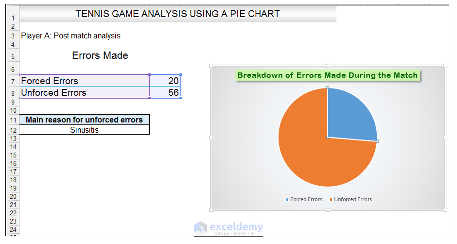
How to Make a Pie Chart in Excel & Add Rich Data Labels to The Chart!

How to Change Axis Values in Excel - Excelchat How to change x axis values. To change x axis values to " Store" we should follow several steps: Right-click on the graph and choose Select Data: Figure 2. Select Data on the chart to change axis values. Select the Edit button and in the Axis label range select the range in the Store column: Figure 3. Change horizontal axis values. Figure 4.

31 How To Label Vertical Axis In Excel

Excel tutorial: How to customize axis labels Instead you'll need to open up the Select Data window. Here you'll see the horizontal axis labels listed on the right. Click the edit button to access the label range. It's not obvious, but you can type arbitrary labels separated with commas in this field. So I can just enter A through F. When I click OK, the chart is updated.

Custom data labels in a chart | Get Digital Help - Microsoft Excel resource

Change axis labels in a chart - support.microsoft.com In a chart you create, axis labels are shown below the horizontal (category, or "X") axis, next to the vertical (value, or "Y") axis, and next to the depth axis (in a 3-D chart).Your chart uses text from its source data for these axis labels. Don't confuse the horizontal axis labels—Qtr 1, Qtr 2, Qtr 3, and Qtr 4, as shown below, with the legend labels below them—East Asia Sales 2009 and ...

Text Labels on a Horizontal Bar Chart in Excel - Peltier Tech Blog

Custom Excel Chart Label Positions - My Online Training Hub Custom Excel Chart Label Positions - Setup. The source data table has an extra column for the 'Label' which calculates the maximum of the Actual and Target: The formatting of the Label series is set to 'No fill' and 'No line' making it invisible in the chart, hence the name 'ghost series': The Label Series uses the 'Value ...

Moving X-axis labels at the bottom of the chart below negative values in Excel - PakAccountants.com

excel - Formatting chart data labels with VBA - Stack Overflow I am developing a dashboard that will have lots of charts, and as the data shown on these charts change, so will the format of the numbers. At the point I am right now, I've run into a problem trying to retrieve the intended format code from the spreadsheet where the data is based on, in the midst of looping through all the series in the chart.

Share :