41 excel chart labels from cells

Custom Axis Labels and Gridlines in an Excel Chart 23/07/2013 · In Excel 2007-2010, go to the Chart Tools > Layout tab > Data Labels > More Data label Options. In Excel 2013, click the “+” icon to the top right of the chart, click the right arrow next to Data Labels, and choose More Options…. Then in all versions, choose the Label Contains option for Y Values and the Label Position option for Left. The labels are (temporarily) shaded … 43 how to convert excel to labels Step 10 Select the worksheet tab from the drop down menu under the "Open Document in Workbook" section and click the "OK" button to open an "Edit Labels" wizard. Step 11 Create and print mailing labels for an address list in Excel Column names in your spreadsheet match the field names you want to insert in your labels.

Plotting Multiple Lines on the Same Figure - Video - MATLAB How to Plot Multiple Lines on the Same Figure. Learn how to plot multiple lines on the same figure using two different methods in MATLAB ®. We'll start with a simple method for plotting multiple lines at once and then look at how to plot additional lines on an already existing figure. (0:20) A simple method for plotting multiple lines at once.

Excel chart labels from cells

Add or remove data labels in a chart - Microsoft Support How to group (two-level) axis labels in a chart in Excel? The Pivot Chart tool is so powerful that it can help you to create a chart with one kind of labels grouped by another kind of labels in a two-lever axis easily in Excel. You can do as follows: 1. Create a Pivot Chart with selecting the source data, and: (1) In Excel 2007 and 2010, clicking the PivotTable > PivotChart in the Tables group on the ... A4 Accounting | Helping you Excel Yourself with spreadsheets One Minute to Excel #24 - 1,000 random dates March 31, 2022. One Minute to Excel #23 - Text numbers to real number again November 25, 2021. One Minute to Excel #25 - Find the breakeven point April 7, 2022. One Minute to Excel #22 - Normalise a budget October 7, 2021.

Excel chart labels from cells. Excel Chart Vertical Axis Text Labels • My Online Training Hub So all we need to do is get that bar chart into our line chart, align the labels to the line chart and then hide the bars. We’ll do this with a dummy series: Copy cells G4:H10 (note row 5 is intentionally blank) > CTRL+C to copy the cells > select the chart > CTRL+V to paste the dummy data into the chart. Accounting Business Management and Tax News | AccountingWEB AccountingWEB is a community site full of useful insights and trend highlights to help tax and accounting professionals improve their practices and better serve their clients. linkedin-skill-assessments-quizzes/microsoft-excel-quiz.md ... Cells A2:D2 are precedents of the formula in cell C4. Cells A2:D2 are dependents of the formula in cell C4. Q107. What is the name given to the numbers in or above each bar in a column chart, as shown? data table; data numbers; data labels; data values; Q108. Which chart type provides the best visual display of the releationship between two ... Free Online Knowledgebase and Solutions - Solve Your Tech Excel formulas present you with a number of options for editing your data. But there is one less commonly used formula that allows you to remove the first character from a cell in Excel. A lot of data that you encounter will not be formatted the way that you need it. Whether a colleague likes to … Read more

How to Create a Chart with Two-level Axis labels in Excel 14/06/2019 · Create a Chart with Two-Level Axis Label Based on Pivot Table. You can also create a Column Chart with two-level axis labels based on a pivot table in your worksheet, just do the following steps: Step1: select your source data, and go to Insert tab, click PivotTable command under Tables group. Basic Excel Tutorial Procedure in Excel 1. Launch Excel. Navigate to your worksheet. 2. Add a column for percentage Change year over year. 3. Add a zero at the topmost cell of the column since it coincides with the Beginning year. 4. Type the following formula. = (B3-B2)/B2 5. Press enter. 6. Create Dynamic Chart Data Labels with Slicers - Excel Campus 10/02/2016 · Typically a chart will display data labels based on the underlying source data for the chart. In Excel 2013 a new feature called “Value from Cells” was introduced. This feature allows us to specify the a range that we want to use for the labels. Since our data labels will change between a currency ($) and percentage (%) formats, we need a ... project time tracker excel Excel For the "Date" column - select a short date format (such as 3/14/12) 2. Select column A and drag its edge to your desired width. Remove the white space at the beginning of the chart. Time Sheet Template for Excel - Timesheet Calculator . Another feature of project time tracking template excel is rows.

How to Color Cells in Excel - Solve Your Tech Use these steps to fill a cell with color in Excel. Open your spreadsheet in Excel. Select the cell or cells to color. Click the Home tab at the top of the window. Click the down arrow to the right of the Fill Color button. Choose the color to use to fill the cell (s.) Our article continues below with more information and pictures for these steps. Publish and apply retention labels - Microsoft Purview ... Solutions > Records management > > Label policies tab > Publish labels If you are using data lifecycle management: Solutions > Data lifeycle management > Label policies tab > Publish labels Don't immediately see your solution in the navigation pane? First select Show all. Follow the prompts to create the retention label policy. 42 how to make labels in excel 2007 This method will introduce a solution to add all data labels from a different column in an Excel chart at the same time. Please do as follows: 1. Right click the data series in the chart, and select Add Data Labels > Add Data Labels from the context menu to add data labels. 2. Right click the data series, and select Format Data Labels from the ... How to Change Excel Chart Data Labels to Custom Values? 05/05/2010 · When you “add data labels” to a chart series, excel can show either “category” , “series” or “data point values” as data labels. But what if you want to have a data label that is altogether different, like this: You can change data labels and point them to different cells using this little trick. First add data labels to the chart (Layout Ribbon > Data Labels) Define the new …

Creating Named Range for a Cell or Range in Excel - ExcelNumber

Tables and Figures - Citing and referencing - Subject ... Tables are numerical values or text displayed in rows and columns. Figures are other illustrations such as graphs, charts, maps, drawings, photographs etc. All Tables and Figures must be referred to in the main body of the text. Number all Tables and Figures in the order they first appear in the text. Refer to them in the text by their number.

Count Cells That Are Not Blank in Excel (6 Useful Methods) | ExcelDemy

What's New: Everything you need to know about the amazing ... How to insert a chart in WPS Spreadsheet 2. How can we add or remove text shading 3. How to insert special symbols in WPS Writer 4. Use format painter to quickly unify text formatting 5. Basic settings on footer and header 6. Wrap text in a cell

Microsoft Excel Tutorials: How to Create a Pie Chart

How to Use Cell Values for Excel Chart Labels 12/03/2020 · Uncheck the “Value” box and check the “Value From Cells” box. Select cells C2:C6 to use for the data label range and then click the “OK” button. The values from these cells are now used for the chart data labels. If these cell values change, then the chart labels will automatically update. Link a Chart Title to a Cell Value

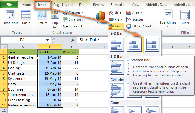
How to make Gantt chart in Excel, step-by-step guidance and templates

How to Make a Chart or Graph in Excel [With Video Tutorial ... Change the size of your chart's legend and axis labels. Change the Y-axis measurement options, if desired. Reorder your data, if desired. Title your graph. Export your graph or chart. 1. Enter your data into Excel. first, you need to input your data into Excel.

Excel label formatting uses cell formatting - Stack Overflow

How to rotate axis labels in chart in Excel? Rotate axis labels in chart of Excel 2013. If you are using Microsoft Excel 2013, you can rotate the axis labels with following steps: 1. Go to the chart and right click its axis labels you will rotate, and select the Format Axis from the context menu. 2. In the Format Axis pane in the right, click the Size & Properties button, click the Text direction box, and specify one direction from the ...

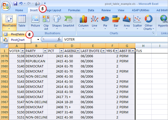
In Search of the Elusive Pivot Table | Dynamic Edge, Inc. | Beyond Tech Support Dynamic Edge ...

Descriptive data analysis: COUNT, SUM, AVERAGE, and other ... 4. While those cells are still selected, hold down the ctrl key and select the data range including the title cell for the proportions in each sex category. 5. Making sure the two cell ranges are still selected, click the "Insert" menu at the top of the Excel window, select the "Column" chart type > 2D (first option).

Share :